Real‑Time Speech with Kaldi’s Online2: A Practical Guide to Low‑Latency Neural Decoding

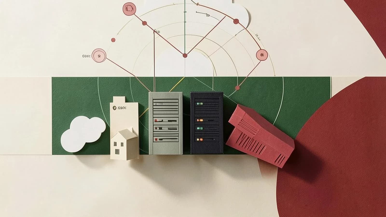
Why Low‑Latency Matters

Voice‑command systems, such as smart assistants or in‑vehicle controls, must respond within 200–300 ms to feel natural. Traditional batch decoding in Kaldi introduces a few seconds of delay and requires the entire utterance to be available. Kaldi’s online2 framework was built to turn a neural acoustic model into a streaming decoder that can process audio on the fly.

What the Pipeline Looks Like

The online2 pipeline is a single process that stitches together four core stages:

• Feature extraction – a streaming MFCC/FBANK extractor that produces features frame‑by‑frame.
• Neural acoustic scoring – a TDNN or LSTM model that maps features to posterior probabilities.
• Beam search – a lattice‑based decoder that keeps the best hypotheses within a configurable beam width.
• Lattice output – a compressed lattice that can be used for downstream tasks or rescoring.

The command online2-wav-nnet3-latgen-faster combines all these steps. It accepts raw WAV files (or a list of file names), runs the neural model, and writes a lattice to disk.

Getting Started: A Minimal Script

# Minimal online decoding example
# Requires: Kaldi compiled with online2, a pre‑trained neural model, and a short wav file.
# Run as: ./run_online.sh /path/to/model /path/to/audio.wav

MODEL_DIR=$1
WAV_FILE=$2
LATTICE_OUT=${WAV_FILE%.wav}.lat.gz

# Verify binaries
if ! command -v online2-wav-nnet3-latgen-faster > /dev/null; then
  echo "Error: online2 binaries missing. Compile Kaldi with online2 first."
  exit 1
fi

# Run decoding
/usr/bin/time -p \
  online2-wav-nnet3-latgen-faster \
    --config=conf/online.conf \
    --beam=12 \
    --acoustic-scale=0.1 \
    --word-symbol-table=$MODEL_DIR/words.txt \
    $MODEL_DIR/nnet3/tdnn_4b_sp/model.json \
    $WAV_FILE \
    > $LATTICE_OUT

# Quick sanity check: lattice should exist and be non‑empty
if [ -s $LATTICE_OUT ]; then
  echo "Lattice written to $LATTICE_OUT"
else
  echo "Decoding failed – no lattice produced"
fi

Replace $MODEL_DIR with the directory that contains words.txt and the neural model. The online.conf file sets feature extraction parameters; the defaults work for most 16‑kHz mono recordings.

Tuning Beam Width and Model Size

The beam width (--beam) controls how many partial paths the decoder keeps. A beam of 10–15 is a good starting point for 16‑kHz input on a modern CPU: you typically see ≈200 ms total latency while keeping word‑error rate (WER) under 10 % on standard test sets.

Increasing the beam improves WER but linearly increases CPU usage and memory. On an embedded ARM Cortex‑A53, a beam of 8 may be necessary to stay below 300 ms latency, even if the WER rises to ~12 %.

Model size matters too. A 4‑layer TDNN with 512 hidden units is a common compromise; deeper or wider networks offer marginal accuracy gains at the cost of higher inference time. If you have GPU acceleration, you can switch to online2-wav-nnet3-latgen-faster-gpu to keep the beam wide without sacrificing latency.

Trade‑Offs on Resource‑Constrained Devices

On a laptop or server you can afford a beam of 20 and a 6‑layer TDNN, achieving ≈5 % WER on LibriSpeech with ≈350 ms latency. On a Raspberry Pi 4, the same model would exceed the CPU budget; you must reduce the beam to 6–8 and possibly prune the model (e.g., via knowledge distillation) to keep latency under 200 ms.

Another consideration is the acoustic-scale parameter. Lowering it (e.g., 0.05) forces the decoder to rely more heavily on the language model, which can help when the acoustic model is noisy but increases decoding time slightly.

Verifying Your Results

After generating a lattice you can evaluate it with Kaldi’s standard scoring scripts:

local/score_kaldi.sh /path/to/exp/online2 /path/to/graph /path/to/test_data

This will produce a WER report. Compare it against the expected range for your model. If the WER is higher than acceptable, try a larger beam or a more robust acoustic model.

Next Steps and Further Optimizations

1. Language‑model rescoring – run latgen-faster-mapped with a 3‑gram or neural LM to shave a few percent off WER.

2. Model compression – use Kaldi’s nnet3-combine or external tools like TensorRT to reduce size and inference time.

3. Profiling – use perf or valgrind to identify bottlenecks in the feature extractor or neural scorer.

4. Hybrid decoding – combine online2 with nnet3-latgen-faster for batch rescoring on the server side.

By iterating on beam width, model size, and post‑processing, you can tailor Kaldi’s online decoder to meet the strict latency and accuracy demands of modern voice‑command applications.