Proceduralism at Scale: Engineering Workflows with Blender Geometry Nodes

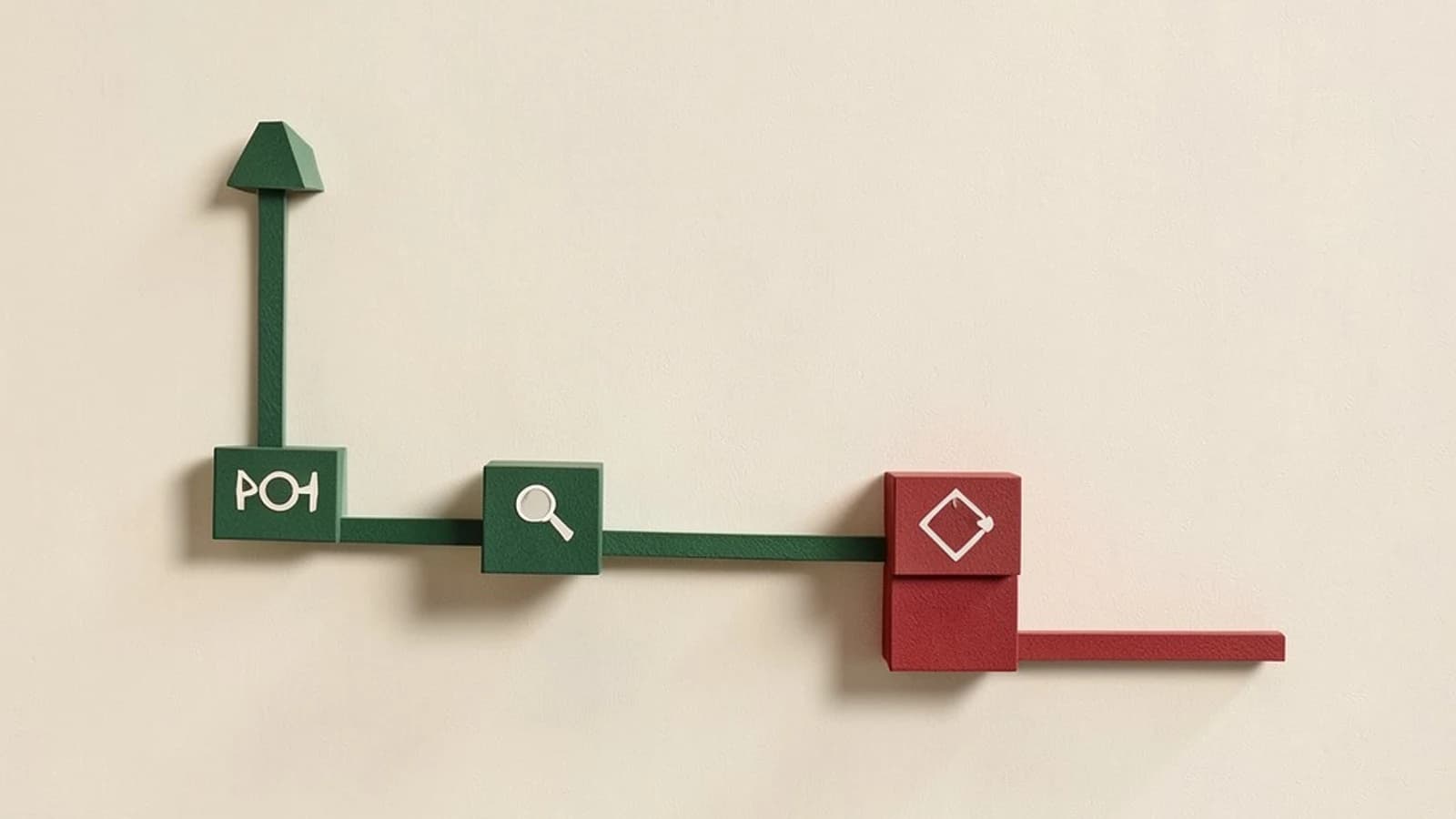
The Bottleneck of Destructive Modeling

Traditional 3D modeling often follows a linear, destructive path: you extrude a face, bevel an edge, and apply a modifier. Once those operations are "applied" or baked into the mesh, returning to a previous decision requires an undo chain or a complete restart. Even the legacy modifier stack in Blender, while non-destructive, operates as a rigid vertical list where the output of one modifier is the input of the next, offering limited control over how data flows between operations.

The shift to Geometry Nodes (introduced in 2.92 and refined in 3.0+) moves Blender from a linear stack to a Directed Acyclic Graph (DAG). The core engineering takeaway is that geometry is no longer just a set of vertices and faces, but a stream of attributes (fields) that can be manipulated, branched, and merged before the final mesh is ever generated.

Fields vs. Attributes: The Logic of Implicit Data

In early versions of Geometry Nodes, data had to be passed explicitly as attributes. If you wanted to move a vertex based on its position, you had to explicitly reference that attribute. Blender 3.0 introduced Fields, a fundamental change in how the system evaluates data.

A Field is essentially a function. Instead of passing a massive list of every vertex position into a node, a field tells the system: "When you get to a specific element, run this calculation to find its value." This lazy evaluation significantly reduces the complexity of the node graph and improves performance, as the system only computes values for the elements currently being processed by the geometry.

Managing Memory with Instance Realization

One of the most critical engineering decisions in a procedural graph is when to Realize Instances. When you use an Instance on Points node to scatter 100,000 trees across a landscape, Blender does not create 100,000 unique meshes. It creates one mesh and 100,000 transform matrices (position, rotation, scale). This is computationally cheap and keeps RAM usage low.

However, instanced data is "read-only." You cannot use a Set Position node to bend a specific tree in that forest because the trees don't technically exist as individual geometry yet. To edit them, you must use the Realize Instances node. This converts the instances into a single, massive mesh. The trade-off is immediate: you gain per-vertex control but lose the memory efficiency of instancing, which can lead to viewport lag or crashes if the polycount exceeds available VRAM.

Worked Example: Creating a Procedural Selection Mask

A common task is applying an effect only to the top-facing parts of a model (e.g., adding snow to a rock). This requires a selection mask based on the surface normal.

Implementation Steps:

1. Input: Start with a Group Input node connected to a Set Position node.
2. Normal Calculation: Add a Normal node. This provides the direction each face is pointing.
3. Dot Product: Connect the Normal node to a Vector Math node set to Dot Product. Set the second vector to (0, 0, 1) (the Z-axis).
4. Thresholding: Pass the result into a Compare node (Greater Than). Set the threshold to 0.5.
5. Application: Plug the output of the Compare node into the Selection input of the Set Position node.

Verification: Open the Spreadsheet Editor (set to Geometry mode). Look for the boolean value generated by the Compare node. If the Z-normal is high, the value should be 1 (True); otherwise, it should be 0 (False). You can verify the visual result by adding a Set Material node using the same selection mask.

The Simulation Zone and State Persistence

Introduced in Blender 3.5, the Simulation Zone allows for feedback loops. In a standard node tree, data flows from left to right. In a Simulation Zone, the output of frame n is fed back as the input for frame n+1.

This enables the creation of custom solvers—such as growth patterns or simple particle physics—without leaving the node editor. However, this introduces a state-management challenge. Because the simulation depends on previous frames, you cannot jump to frame 100 without calculating frames 1 through 99. This makes the Cache settings vital; long simulations can consume gigabytes of RAM if not baked to disk or limited via the Cache Mode settings.

Limitations and Constraints

Constraint	Technical Impact	Mitigation
32-bit Index Limit	Extremely high instance counts may hit the depsgraph limit.	Split geometry across multiple GN modifiers.
Version Locking	Groups using newer nodes won't work in LTS versions.	Use standardized node groups and avoid beta-only nodes.
Debugging	No step-through debugger for node logic.	Use the Viewer Node and Spreadsheet Editor for data inspection.

Closing Action

To transition from destructive to procedural workflows, start by replacing your most repetitive tasks—like scattering objects or creating variations of a prop—with a Geometry Node tree. Use the Spreadsheet Editor to treat your geometry as data rather than just a visual mesh, and always defer Realize Instances until the absolute last step of your graph to maintain performance.