LinkedIn People You May Know: A Graph‑Based Scoring Walkthrough

The problem: why a connection feels “just right”

When you log into LinkedIn and see a list of people you might know, the platform is trying to surface profiles that are likely to be relevant to your professional network. The underlying task is a similarity search over a massive social graph: given a user , find other users  whose connection pattern and profile attributes make them good candidates for a new link.

How the score is built: a weighted graph model

LinkedIn treats its network as a directed, weighted graph G = (V, E) where each node v ∈ V is a member and each edge e = (u, w) ∈ E represents a connection. Edge weights can capture interaction frequency, endorsement strength, or simply be set to 1 for an unweighted link.

The similarity score between a target user u and a candidate v is typically a linear combination of several signals:

1. Mutual‑connection term – the number of shared neighbours, often normalized to reduce bias toward high‑degree users.
2. Attribute overlap – shared skills, groups, companies, or educational institutions.
3. Recency/activity – recent interactions, profile updates, or content engagement.
4. Network‑depth penalty – a factor that diminishes the score for candidates that are already far away in the graph (e.g., friends‑of‑friends‑of‑friends).

A simplified formula that captures the first two components looks like this:

score(u, v) = α * (|N(u) ∩ N(v)| / sqrt(deg(u) * deg(v)))  + β * (shared_skills(u, v) / max_skills)  + γ * recency_signal(u, v)

where N(x) is the neighbour set of x, deg(x) its degree, and α, β, γ are tunable weights.

Worked example: computing a match score

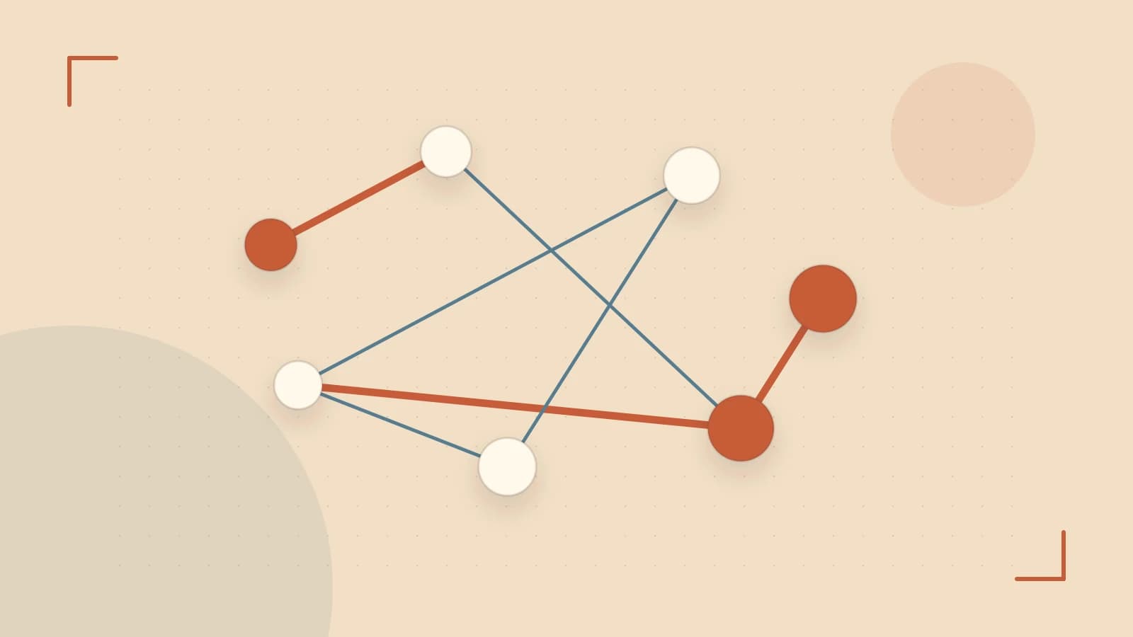
Consider a tiny sub‑graph with four users:

• A (you) is connected to B, C, and D.
• B is connected to A and E.
• C is connected to A, E, and F.
• D is connected only to A.
• E and F are not connected to A.

Assume the following attribute data (skills):

• A: {Python, SQL, Leadership}
• B: {Python, Java}
• C: {SQL, Leadership, MachineLearning}
• D: {Marketing}
• E: {Python, MachineLearning}
• F: {Leadership, Marketing}

Using α = 0.6, β = 0.3, γ = 0.1 and setting the recency signal to 0 for all pairs (no recent interaction), we compute the score for each candidate versus A.

Mutual‑connection component (normalized):

• |N(A)∩N(B)| = 0 → term = 0
• |N(A)∩N(C)| = 0 → term = 0
• |N(A)∩N(D)| = 0 → term = 0
• |N(A)∩N(E)| = 0 → term = 0
• |N(A)∩N(F)| = 0 → term = 0

Because A shares no two‑hop neighbours with any of the candidates in this tiny graph, the mutual‑connection term contributes nothing.

Shared‑skill component (skills overlap divided by max possible skills, here 3):

• shared_skills(A,B) = {Python} → 1/3 ≈ 0.33
• shared_skills(A,C) = {SQL, Leadership} → 2/3 ≈ 0.67
• shared_skills(A,D) = {} → 0
• shared_skills(A,E) = {Python} → 1/3 ≈ 0.33
• shared_skills(A,F) = {Leadership} → 1/3 ≈ 0.33

Plugging into the formula (γ = 0.1, recency = 0):

• score(A,B) = 0.6*0 + 0.3*0.33 + 0.1*0 ≈ 0.10
• score(A,C) = 0.6*0 + 0.3*0.67 + 0.1*0 ≈ 0.20
• score(A,D) = 0
• score(A,E) = 0.10
• score(A,F) = 0.10

Thus, C receives the highest score and would appear first in the “People You May Know” list for A, even though they share no mutual connections, because of overlapping skills.

Trade‑offs and limitations

While the mutual‑connection term is powerful, relying heavily on it can reinforce existing network homophily: users with dense, tightly‑knit clusters keep seeing similar profiles, reducing exposure to diverse industries or geographies. Normalizing by degree (as in the sqrt(deg(u)·deg(v)) factor) mitigates bias toward super‑connectors but may penalize legitimate professionals who maintain large, genuine networks.

Another practical constraint is scale. Computing exact similarity for all pairs in a graph with hundreds of millions of nodes is infeasible. Production systems therefore use approximate nearest‑neighbor techniques (e.g., locality‑sensitive hashing on skill vectors) or graph‑sampling strategies to limit the candidate set before applying the full score.

Actionable takeaways for engineers

1. Start with a clear signal hierarchy: mutual connections → attribute overlap → activity.
2. Implement a simple baseline score (like the formula above) on a small, synthetic graph to validate ranking logic before moving to approximations.
3. Monitor homogeneity metrics (e.g., entropy of recommended industries) to detect over‑reliance on any single signal.
4. When scaling, experiment with locality‑sensitive hashing on skill embeddings to retrieve a shortlist, then apply the full weighted score only to that list.
5. Provide a knob for product teams to tune α, β, γ based on A/B test results, and log the chosen weights for reproducibility.

By grounding the recommendation process in a transparent, weighted‑graph model and validating it on a manageable sub‑graph, you can iterate quickly while keeping an eye on the broader impacts of network bias and computational cost.